A couple posts ago, I described the machine learning model that we developed to predict the extent of cropland irrigation worldwide. This post is a collection of all the things I learned about Google Earth Engine that went into running a global-scale model successfully.
GEE: Strengths and Weaknesses
First, it helps to understand Google Earth Engine itself on where it’s strong and where it’s weak. GEE is a cloud service for geospatial data processing. We processed terabytes of satellite data for our model. This means you don’t have to worry about setting up the relevant compute cluster, or its associated software. This is a huge win.
GEE provides a set of APIs to access its service, which is very close to the problem domain of geospatial data. The APIs are well-documented and there are additional tutorials available from the community as well as past conferences. However, you may have to know two different languages, JavaScript and Python, as I will explain in a bit.
GEE has a functional, map-reduce programming model. i.e., the programmer is expected to know and use map-reduce like APIs to distribute processing. The system evaluates lazily, creating a lineage graph back to the source when it actually sees an output. In this way, GEE is closer to Apache Spark than say Pandas in terms of its data processing model. This can be a strength as well as a weakness. If you’re a data scientist, wrapping your head around functional concepts can be a learning curve and a distraction.
Besides compute, GEE also hosts many curated and cleaned geospatial datasets. This includes satellite imagery, climate, ocean and land datasets. Some of them are primary, but there are also derived datasets such as averages and vegetation indices. This allows researchers to focus on actually doing research, instead of wrangling with the data and making it available for computation. This doesn’t mean that model development is a cake-walk, but it definitely takes some of the burden off. This is again a big win: we once tried to process MODIS datasets ourselves using its heg tool and it was a nightmare.
GEE also allows machine learning. However, the choice of models for supervised classification is limited to SVM, CART, random forest and naive Bayes. The way I made sense of it is: you’re limited to algorithms that are parallelizable. You can always grow trees in a forest, or compute probabilities, independently and in parallel. This is practically not a big limitation because random forest is a robust algorithm. GEE also allows clustering and computing statistics, but I didn’t use them for this project. A second problem is that it was not easy to tune a model for hyperparameters. What is the best tree depth, or even the best number of trees? Where should the classification threshold be? We had to ship data out from GEE to do these in R, as I will explain more in the strategy section.
To ease development experience, GEE has an integrated browser-based IDE. The IDE has a way to write code and look at results on a map or a graph. It also shows any pictures or tables you’ve saved within GEE. I found the IDE useful at the two ends of the model development lifecycle. It was useful at the beginning, when we quickly had to explore data and maps. It was also useful at the end, when we developed powerful, interactive apps to showcase results. This is a JavaScript environment with a rather bad limitation: I did not find any way to invoke code written here from outside of the IDE. This means I could not automate workflows here.
A related quirk feature about GEE is that it has two modes of running computations: an interactive mode and a batch mode. By default, what you do on the browser IDE runs interactively and has a timeout set at 5 minutes. On the other hand, if you create a task, it goes into a queue and runs in batch mode. Batch jobs can use more resources. Many of our jobs ran for hours, and sometimes waited in the queue for a day. I didn’t know about this mode, and I wasted a few days trying to create a global model within the IDE that could finish in 5 minutes (what was I thinking?).
GEE also offers a Python API you can run from your laptop. I used this for actual running of the model. This means you might have to rewrite code from JavaScript to Python, although the APIs are so similar that it is not a big deal. You will miss visualizing the results quickly, which is possible in the browser-based IDE. As an alternative, I wrote results and visualized them back in the IDE. If you also follow our strategy and do model selection and tuning in R, there are three languages in the mix now.
GEE can store results within itself as GEE assets. When you store a map there, it also stores maps at other resolutions, in what is called pyramiding. This allows GEE to pick the right resolution map when it’s read for processing. You can group images and tables together into collections, and add metadata such as source and time period. For assets, GEE readily shows image bands and their resolution as well as a thumbnail map.
A significant weakness of GEE is that it’s new and closed source, and there is not much in the way of community libraries or packages. It’s pretty much a niche product right now. I found the original GEE paper to be extremely useful in understanding its design. There is also a profiler built into the browser-based IDE that can shed light when things are slow.
Useful Domain Concepts
To be successful with geospatial machine learning, you’ll need to know some domain concepts. Here is a list of concepts I found most useful.
Vectors vs. rasters: A raster is like a JPEG file, where you store values for each square in a grid of squares. A vector is like an SVG file, where you specify points, lines and polygons to draw a picture. GeoTIFF is a raster file format, that can hold multiple rasters or bands. ShapeFile and GeoJSON files can store vectors.
Satellite terminology: Satellites capture pictures at a certain spatial resolution (say 500m). This means one pixel in its picture corresponds to 500m, so you cannot hope to see anything finer than that. This is similar to optical zoom in digital cameras. Satellites also revisit the same place as they revolve around the earth. How frequently they come back corresponds to temporal resolution. MODIS and LANDSAT are two key satellites for historical data, but Sentinel is newer. MODIS satellites take pictures more frequently, but their spatial resolution is 500m. LANDSAT is less frequent, but its resolution is much better at 30m. The way satellites take pictures is also different: they sense the area in various bands of the electromagnetic spectrum: infra-red, near infra-red, red, blue, and so on. Instead of using the band readings directly, researchers have taken ratios of bands to infer whether land is forested or cropped. NDVI is such a vegetation index, quite literally (Band 5 - Band 4) / (Band 5 + Band 4) on LANDSAT 4-7.
Cartographic projections and radial area measures: Because Earth is spherical but maps are flat, they approximate the curvature differently. For example, Mercator projection simply flattens the globe to a square like you’d roll a dough ball, so it stretches the poles. If your maps have different projections, it is important to standardize on one projection. Otherwise the pixels can be off and can create problems. MODIS uses sinusoidal projection, for example. On GEE, different projections are not a problem because it reprojects maps internally, based on the output projection.
Spatial resolution is often given in arc-degrees and minutes, which can be confusing. This also comes from the way Earth is: spherical. The best way to understand is to imagine a circular slice of the Earth and a covered light bulb at its center, so that it’s lighting up only a small arc of the circle. The angle the arc makes at the center is the number you’re seeing, and that’s why it’s given in degrees, minutes or seconds.
Features vs. images: On GEE, a feature is a geometry (such as a point, line, polygon) along with a dictionary of properties. The geometry is optional, so if you simply want to create a table, ignore the geometry and make the column names the dictionary keys. An image is a raster. GEE also allows you to group them into feature- and image-collections. Some operations on GEE, such as training a random forest classifier, work only on feature collections.
Our Model Development Strategy
GEE is a shared service, so there are limits to how much memory you can use. At 4km resolution, Israel was the largest country we could train our model on GEE. Yet, our aim was to create a global model. Even if we could get there, we had no way to look at feature importances1 or tune for the best model and its hyperparameters. This stalled our project for a couple weeks. That’s when we decided to download a sample and do model development offline using the R ecosystem. We wrote code to take a random global sample of 10,000 points from GEE. We downloaded this sample to our laptop and used R to select and tune our model. The caret package makes it very easy to do this. Once we had our model and hyperparameters, we could simply plug in the values on GEE and continue our work there.
So, here is our recipe for large-scale ML models on GEE:
Step 1: Take a random sample. All your features should be in this sample. If there is class imbalance, keep doubling sample size until it captures enough variability in the minority class.
Step 2: Come up with your model outside of GEE. Don’t bother with algorithms that are not supported on GEE, because your final model needs to run on GEE. Use a high-level statistical environment like R and caret. The output will be your final choice of classification algorithm and its tuned hyperparameters.
Step 3: Predict on GEE with your model. You can code the algorithm and hyperparameters based on what you got in the previous step. Try predicting on the whole world first. If it fails, start dividing into continents, then countries. Use probability mode (i.e. soft prediction) to intelligently set binary threshold. When we developed the project, there was no way to save a trained model, so it had to be trained for every new run.
Reducing Amount of Data to Process
It helps immensely if you can intelligently reduce data to process:
- GEE allows you to specify masks to ignore certain areas of a map. We used this to ignore oceans, Antarctica and Pacific Islands.
- Our resolution is at 8km not only to match with the labels, but because it also reduced data to process and let us focus on the data science aspects of it. Area grows quadratically, so expect to process 4 times more data if you go for half the resolution.
- We pre-processed and created intermediate tables where we had to calculate time averages, i.e. average over the whole year. We stored these results and fed them to the model as features. We did not try to the time-averaging during the actual model prediction.
- We created a hybrid model. We developed a more sophisticated model for lands already identified as croplands, but still had a coarse model that ran globally. We could probably also reduce data if we filtered out areas outside the usual NDVI range for croplands. We did not try this in our project.
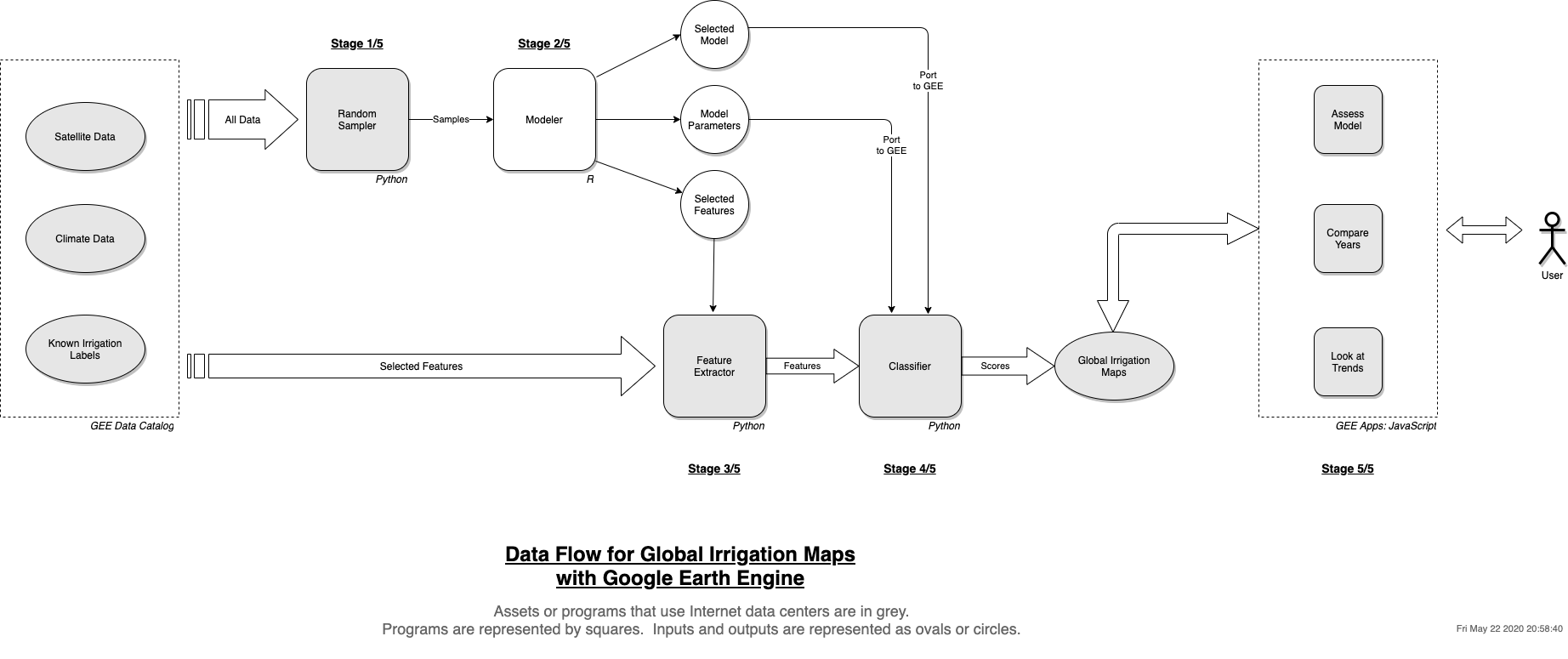
The following diagram shows our final model pipeline.
Tips and Caveats
Finally, here are some other assorted tips for a successful GEE project.
- Save your vectors in GeoJSON and your images in GeoTIFF formats.
- Remember that GEE works backwards from output: the projection, scale and extent are propagated back to the sources, so that it has less data to process.
- Use the browser-based IDE at the ends of the project. Do initial exploration and prototyping there. Also use it to create interactive apps when you do your final maps.
- Data transformations can become a long chain. Always visualize the results at every step. Be sure each step does what it is supposed to do.
- Don’t use
forloops, usemap()calls in Python and JavaScript instead. This parallelizes the processing and makes it fast. - Remember that GEE keeps everything on the server. Simply calling
print(object)will not work in Python. Instead you should doprint(object.getInfo()). - Budget some time to know your datasets: their spatial and time resolution, first and last years. Be sure to actually look at it on a map and note whether any map areas are masked out within the dataset.
- Join the GEE developers mailing list to ask questions. It’s a niche product and that’s your refuge if you run yourself into a corner. The error messages can sometimes make no sense if you don’t understand its design.
Closing Remarks
Developing our project on GEE was hard and frustrating. When we started the project, I knew nothing about geospatial data or domain, nor did I know anything about Google Earth Engine. We had only 14 weeks to show results. Because of my software engineering and big data background, some parts of the project were easier: I could write functional programs, I could make sense out of error messages and debug my way out of them, and I could juggle multiple languages and programming environments. Still, there were many challenges given the goal of the project, and there were many days when I asked myself why I even set out to do this. Google Earth Engine seemed like a beast I was constantly wrestling with. Even when I could figure out how to do something on it, our project’s global scope meant I would inevitably run into GEE limits. Having a manual offline tuning step meant one-click automation of the model was not easy. We also had some wasted detours in trying to export data and running on a Spark cluster, or processing satellite data tiles ourselves with R and Python libraries. On top of all this, there was family and office work that needed our time and attention.
Ultimately, I’m very satisfied that we could accomplish what we originally set out to do. Despite its quirks, I honestly think GEE makes large-scale geospatial research possible and accessible. The alternatives I tried are much worse, and once you get a hold of GEE, you can be very productive and focus on solving geospatial problems. I’m glad and grateful that Google created this product and made it available to the research community.
Our model source code is available, along with additional documentation in the repository README.
–
1 This has since been corrected: their SmileRandomForest classifier now has an API to show feature importances.